Create Advanced Filter|Financial calculation|Balance method

Create an Excel Advanced Filter

Here are the steps for setting up your data, and creating an Advanced Filter.

1. Set up the database

1. The first row (A1:D1) has headings. Each column must have a unique heading -- duplicate headings will cause problems when running an Advanced Filter.
2. Subsequent rows contain data.
3. There are no blank rows within the database.
4. There is a blank row at the end of the database, and a blank column at the right.

2. Set up the Criteria Range (optional)

In the criteria range for an Excel advanced filter, you can set the rules for the data that should remain visible after the filter is applied. You can use one criterion, or several.

1. In this example, cells F1:F2 are the criteria range.
2. The heading in F1 exactly matches a heading (D1) in the database.
3. Cell F2 contains the criterion. The > (greater than) operator is used, with the number 500 (no $ sign is included).

After the Excel advanced filter is applied, orders with a total greater than $500 will remain visible.

Other operators include:
< less than
<= less than or equal to
>= greater than or equal to
<> not equal to

3. Set up the Extract Range (optional)

If you plan to copy the data to another location, you can specify the columns that you want to extract. If you want to extract ALL columns, you can leave the extract range empty for the Excel advanced filter.

1. Select the cell at the top left of the range for the extracted data.
2. Type the headings for the columns that you want to extract. These must be an exact match for the column headings, in spelling and punctuation. The column order can be different, and any or all of columns can be included.

4. Apply the Excel Advanced Filter

1. Select a cell in the database.
2. On the Excel Ribbon's Data tab, click Advanced, to open the Advanced Filter dialog box

3. You can choose to filter the list in place, or copy the results to another location.
4. Excel should automatically detect the list range. If not, you can select the cells on the worksheet.
5. Select the criteria range on the worksheet
6. If you are copying to a new location, select a starting cell for the copy
   Note: If you copy to another location, all cells below the extract range will be cleared when the Advanced Filter is applied.
7. Click OK

Or, step by step following:

How to create advance filter?

Type your perfect data and copy to header from another location > write to any data > short & filter > click on advance > select list range > select criteria range > click on copy to another location > select copy to cell > ok.

Financial calculation in excel

To illustrate Excel's most popular financial functions, we consider a loan with monthly payments, an annual interest rate of 6%, a 20-year duration, a present value of $150,000 (amount borrowed) and a future value of 0 (that's what you hope to achieve when you pay off a loan).

We make monthly payments, so we use 6%/12 = 0.5% for Rate and 20*12 = 240 for Nper (total number of periods). If we make annual payments on the same loan, we use 6% for Rate and 20 for Nper.

Pmt

Select cell A2 and insert the PMT function.

Note: The last two arguments are optional. For loans the Fv can be omitted (the future value of a loan equals 0, however, it's included here for clarification). If Type is omitted, it is assumed that payments are due at the end of the period.

Result. The monthly payment equals $1,074.65.

Tip: when working with financial functions in Excel, always ask yourself the question, am I making a payment (negative) or am I receiving money (positive)? We pay off a loan of $150,000 (positive, we received that amount) and we make monthly payments of $1,074.65 (negative, we pay).

Rate

If Rate is the only unknown variable, we can use the RATE function to calculate the interest rate.

Nper

Or the NPER function. If we make monthly payments of $1,074.65 on a 20-year loan, with an annual interest rate of 6%, it takes 240 months to pay off this loan.

We already knew this, but we can change the monthly payment now to see how this affects the total number of periods.

Conclusion: if we make monthly payments of $2,074.65, it takes less than 90 months to pay off this loan.

Pv

Or the PV (Present Value) function. If we make monthly payments of $1,074.65 on a 20-year loan, with an annual interest rate of 6%, how much can we borrow? You already know the answer.

Fv

And we finish this chapter with the FV (Future Value) function. If we make monthly payments of $1,074.65 on a 20-year loan, with an annual interest rate of 6%, do we pay off this loan? Yes.

But, if we make monthly payments of only $1,000.00, we still have debt after 20 years.

Or, following formula:

How can we financial calculation in excel?

Formula > function library > insert > function > financial > pmt/ipmt/ppmt > type your rate, nper, pv > ok.

–: Following the chart below :–

Principle	Rate	Term	Per	Pmt	Ipmt	Ppmt
100,000	11%	12	12

Balance method Description

Returns the depreciation of an asset for a specified period using the fixed-declining balance method.

Syntax

DB(cost, salvage, life, period, [month])

The DB function syntax has the following arguments:

• Cost    Required. The initial cost of the asset.
• Salvage    Required. The value at the end of the depreciation (sometimes called the salvage value of the asset).
• Life    Required. The number of periods over which the asset is being depreciated (sometimes called the useful life of the asset).
• Period    Required. The period for which you want to calculate the depreciation. Period must use the same units as life.
• Month    Optional. The number of months in the first year. If month is omitted, it is assumed to be 12.

Remarks

• The fixed-declining balance method computes depreciation at a fixed rate. DB uses the following formulas to calculate depreciation for a period:
  (cost - total depreciation from prior periods) * rate
  where:
  rate = 1 - ((salvage / cost) ^ (1 / life)), rounded to three decimal places
• Depreciation for the first and last periods is a special case. For the first period, DB uses this formula:
  cost * rate * month / 12
• For the last period, DB uses this formula:
  ((cost - total depreciation from prior periods) * rate * (12 - month)) / 12

Example

Copy the example data in the following table, and paste it in cell A1 of a new Excel worksheet. For formulas to show results, select them, press F2, and then press Enter. If you need to, you can adjust the column widths to see all the data.

Data	Description
$1,000,000	Initial cost
$100,000	Salvage value
6	Lifetime in years
Formula	Description	Result
=DB(A2,A3,A4,1,7)	Depreciation in first year, with only 7 months calculated	$186,083.33
=DB(A2,A3,A4,2,7)	Depreciation in second year	$259,639.42
=DB(A2,A3,A4,3,7)	Depreciation in third year	$176,814.44
=DB(A2,A3,A4,4,7)	Depreciation in fourth year	$120,410.64
=DB(A2,A3,A4,5,7)	Depreciation in fifth year	$81,999.64
=DB(A2,A3,A4,6,7)	Depreciation in sixth year	$55,841.76
=DB(A2,A3,A4,7,7)	Depreciation in seventh year, with only 5 months calculated	$15,845.10

Or, following formula:

How to Balance Method?

Formula > function library > insert > function > financial > db > type cost, salvage, life, period > ok.

–: Following the chart below :–

Cost	Life	Term	Per	Salvage	Db
60,000	5	3	2	40,000

How to Consolidate Data in Excel

There are many ways to consolidate data in Microsoft Excel. You can use the Table feature and its associated filters to filter a list so it shows only those items you are interested in seeing and you can create PivotTables to look at your data in different ways. You can also consolidate large amounts of data into a summary form which can show you as much or as little of your data as you want to see. In this post, I'll show you how to use the Consolidate data feature in Excel to take data from a series of worksheets - or workbooks - and summarize them into a single worksheet.

Work with multiple data sets

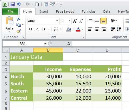
Consider the situation where you have data for twelve months of your business stored one month per sheet in an Excel workbook. If each sheet contains that month's data and if it is laid out in the same arrangement of columns and rows then you can summarize this full year of data into a single sheet using the Consolidate tool.

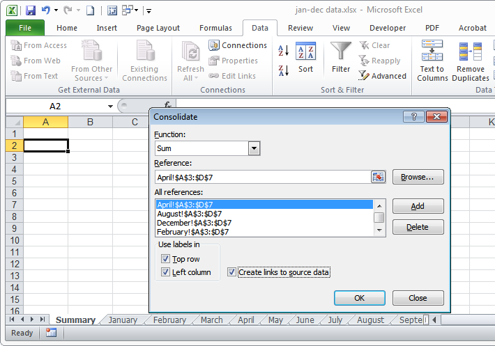
To do this select an empty sheet in the workbook - add a new one if necessary - and click in it. Choose Data > Consolidate to view the Consolidate dialog. Here you will select the function to analyze your data and the references or ranges that you want to consolidate. For our data we want to add the values so we'll set the Function to Sum. However we could have chosen any of these 11 functions: Sum, Count, Average, Max, Min, Product, Count Numbers, StdDev, StdDevp, Var and Varp.

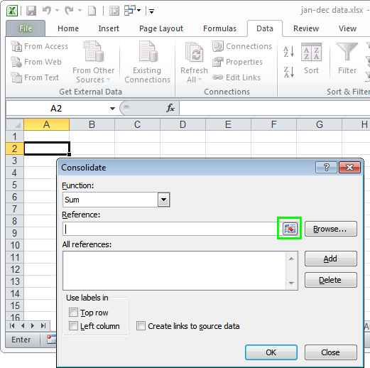
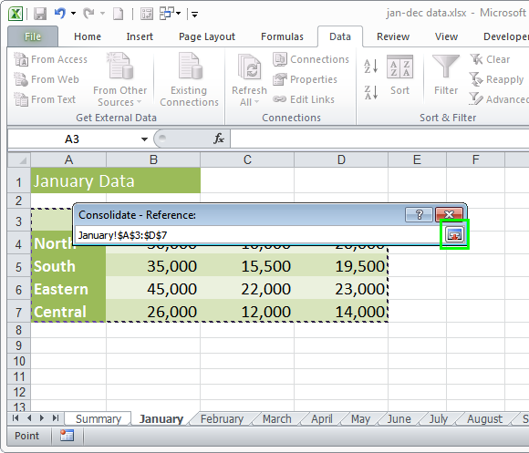
Click in the Reference area and click the Expand/Collapse button to its immediate right. Select over the first data range to consolidate - to do this you will need to click the Sheet tab and then drag over the data including the row and column headings.

Back in the Consolidate dialog, click Add to add this first set of data to the consolidation dialog. Continue and add the second and each additional set of data to the References section of the dialog. Provided you have the same range of data on each of your worksheets and they are all in the same position all you will need to do is to click the Worksheet tab and the range will already be selected for you so it's not as big a job as it might seem.

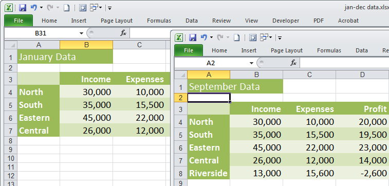
The ranges you consolidate do not necessarily have to be of the same size in each worksheet. So the number of rows or the number of columns or the number of rows and columns might be different from sheet to sheet. For example, if we had opened a new office in a September, we would need to expand the range selected in September to account for the additional rows of data for that new office and we would then continue to do that for every worksheet that contained those extra rows.

Top Tip

You can name your ranges before you start the Consolidation process. To do this, select a range and type a name for it into the Name box at the far left of the Formula bar. If you name each range then, when you create the consolidation, place your cursor in the Reference field, press F3 and then choose the range from the list in the Paste Name dialog. This way you can give each range a descriptive name and you won't need to remember later what you had entered in Sheet1, cells A3:F40.

You'll see that the worksheets appear in the All References panel in alphabetical order. Check that you have all the references there before you continue. Select the Use labels in: Top Row and Left Column checkboxes. Select the Create links to source data check box and click Ok.

The consolidated data

When you click Ok, Excel summarizes all the data into your new sheet. You will see grouping tools down the left of the screen which you can use to display and hide the data.

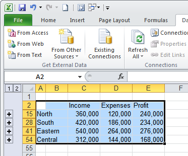
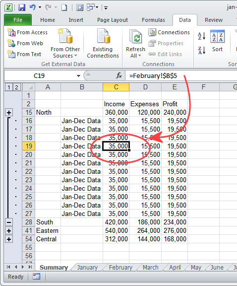
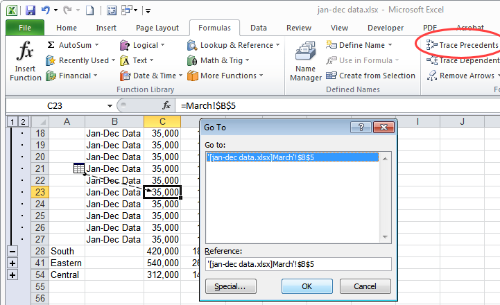
If you chose "Create links to source data" then the data is linked to the original cell containing it. To see this, click in a cell with the data (not a sum function) and you will see a reference to the sheet and cell that contains that data.

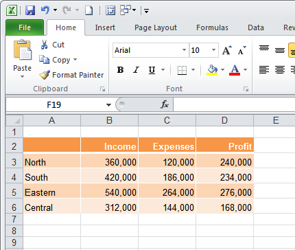
If you did not choose "Create links to source data" the consolidation is simply a summary of the data without any details so there is no grouping applied and the results are summarized only.

Top Tip

As this data is linked you can use the Trace Precedents option to go to the cell containing that data. To do this, click in the cell that contains the data you want to view. Click Formulas tab > Trace Precedents. Because the precedent cell is on a different worksheet hold your mouse over the black arrow head till the mouse cursor turns into a hollow white arrow. Double click to open the Go To dialog - the cell reference will be automatically listed there. Click it and click Ok to go to that cell.

Format the data

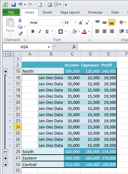
You can format the data in the summary worksheet as you would in any regular Excel file. You'll find that the second column of data shows the name of the workbook that contains the data. You can hide this column, if desired, by right clicking it and choosing Hide. This simply hides the column so the data is there should you need to refer to it later on.

Different workbooks

One of the benefits of using this Consolidation tool is that the data does not need to be in a single workbook. Instead, if you have a series of workbooks each of which contains a similar arrangement of data for different periods of time, you can consolidate all these using this tool.

To do this you would use the same process as before and select an empty worksheet or click Insert > Insert Sheet to include a new worksheet in a workbook. Choose the Consolidate tool and this time instead of selecting a sheet in the current workbook, click the Browse button to open a different workbook.

Now select the references to use in that particular workbook. Repeat for each workbook containing the data you are interested in viewing. I find it easier to switch between open workbooks when I add the Switch Windows button to the QAT (Quick Access Toolbar).

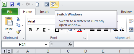
If you select the Create Links to Source Data checkbox then, when you create your consolidation, the connection will be live so that changes in the underlying worksheets and workbooks will be reflected in the consolidated data. In addition, the second column of the summary will display the workbook name. The tip about using Trace Precedents also works to quickly take you to the workbook if it is open already, but will fail if it is not.

Or, following formula:

How to create a data consolidate?

At first, open four work sheet > type perfect data (above) for consolidate into one two three work sheet and four work sheet > select without number area of fourth work sheet > data > data tools > consolidate..

a)click on function key - - - - sum

b)put the cursor of reference & select your 1^st sheet number data area > click on add.

c)select your 2^nd sheet number data area > click on add.

d)select your 3^rd sheet number data area > click on add > ok.

–: Following the chart below :–

Date:                                                 Kolkata Branch

Serial number	Item	January	February	March
1	Pc	100	200	300
2	Cd	300	400	500
3	Hard disk	600	700	800